The bias-variance tradeoff is one of the main buzzwords people hear when starting out with machine learning. Basically a lot of times we are faced with the choice between a flexible model that is prone to overfitting (high variance) and a simpler model who might not capture the entire signal (high bias). To better understand the trade-offs I’m going to do a little experiment inspired by an exercise in the book Learning From Data. We’ll take a target function - a polynomial of some degree, add some noise, and then generate a number of training examples. Then we will fit two different functions: the first a polynomial of degree 2 and the second a polynomial of degree 10. We will then devise an overfit measure and see how well our two models are at capturing the signal of the original target function as we vary the number of examples, the amount of noise and the degree of the original functions.
Let \(Q\) be the degree of our target polynomial \(f\), \(N\) - the number of noisy examples generated and \(\sigma\) the standard deviation of the noise. We will now fit a second degree polynomial \(g_2\) and a tenth degree polynomial \(g_{10}\) to the data we generated while varying \(Q\), \(N\), and \(\sigma\) and see what insights we can get into overfitting. For a fixed triple \((Q, N, \sigma)\) the overfit measure will be \(E_{out}(H_{10}) - E_{out}(H_2)\) - the difference in out of sample error in fitting the data with a tenth and a second degree polynomial averaged over \(500\) runs - the averaging is necessary since, as we shall see, the variance of \(E_{out}(g_2)\) and \(E_{out}(g_{10})\) can be high.
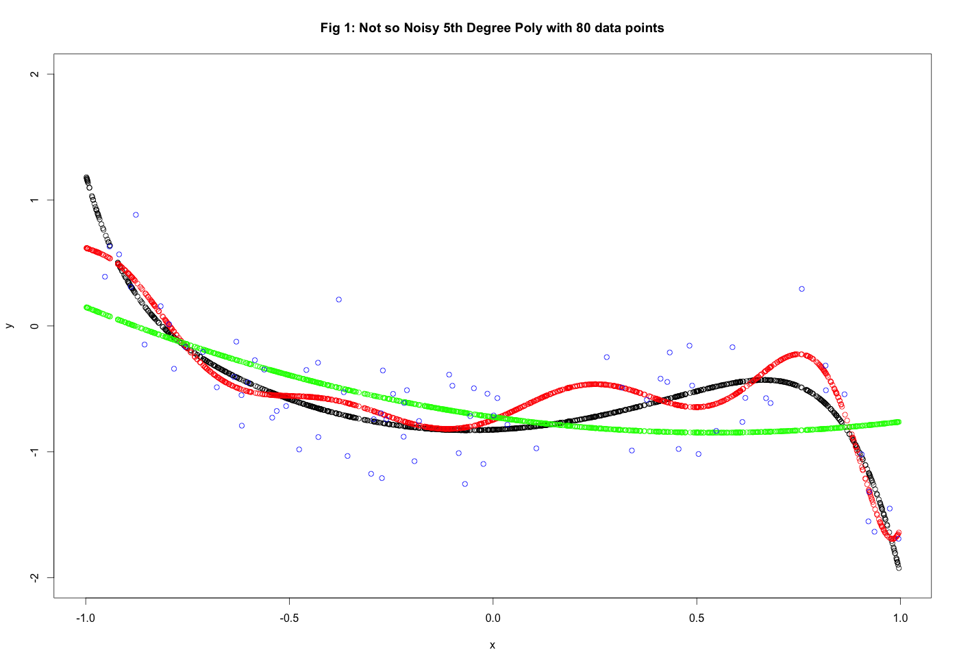
To begin let’s choose \(Q = 10, N = 80, \sigma^2 = .1\). The results of out fit can be seen in Figure 1 and the code generating the plot can be found right belowe the plot. Keep in mind that as we are fitting the models we do not have access to the original target function in black. So what we can tell just by looking at the picture and numbers: We see that \(g_{10}\) performs better than \(g_2\) – we get \(E_{out}(g_2) = 0.0970\) and \(E_{out}(g_{10}) = 0.0221\). For the second degree polyomial fit the main contributor to \(E_{out}\) is the bias - the model cannot capture the complexity of the target function - it does however do a good job of not fitting the noise. The opposite is true for \(g_{10}\). In this case the model does have enough complexity to fit the data but since noise is present it fits some of the noise in as well - thus the variance of the model increases.
The colors in the plosts are as follows: black denotes the original target function, green is the second degree fit \(g_2\), red is the 10th degree fit \(g_10\) and the blue dots are the noise training examples.
library(polynom)
set.seed(127)
q = 10 #degree of poly
n = 80 #number of examples
s = .1 #this is really sigma squared
x <- runif(n, min = -1, max = 1)
poly <- polynomial(rnorm(n = q+1)) #poly
epsi <- rnorm(n) #noise
y <- predict(poly, x) + sqrt(s)*epsi #values of poly +noise
df <- data.frame(x, y)
model_2 <- lm(y ~ poly(x,2), data = df)
model_10 <- lm(y ~ poly(x, 10), data = df)
#now we want E_out
test <- runif(1000, min = -1, max = 1)
testdf <- data.frame(test)
colnames(testdf)[1]<-"x"
plot(test, predict(poly,test), ylim = c(-2,2), xlab = "x",
ylab = "y", main = "Fig 1: Not so Noisy 5th Degree Poly with 80 data points")
newy_2 <- predict(model_2, newdata = testdf)
newy_10 <- predict(model_10, newdata = testdf)
points(test, newy_10, col = "red")
points(test, newy_2, col = "green")
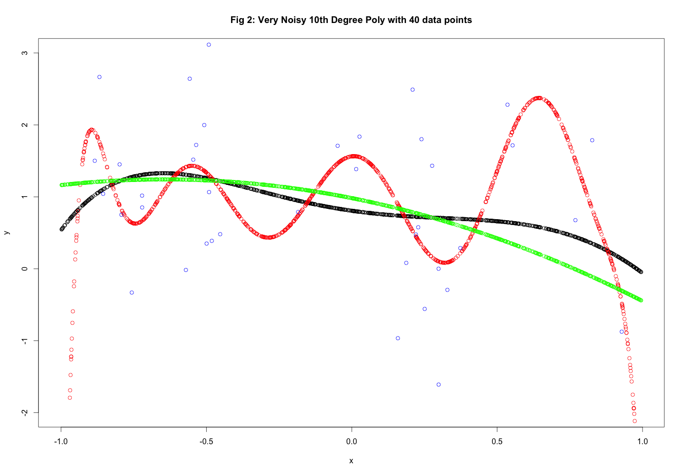
points(x, y, col = "blue")One would thus expect \(g_{10}\) to perform more poorly as amount of noise increases and the number of examples decreases and this will in fact be the case. Let’s do an examples with \(Q = 5, N = 40, \sigma^2 = 1\). This is seen in Figure 2. In this case we get \(E_{out}(g_2) = .061\) and \(E_{out}(g_{10} = 1.12\). \(g_2\) is the clear winner here - it still showcases some bias but it deals with the noise much better. \(g_{10}\) fits too much of the noise leading to an increase in the variance and thus an increase in \(E_{out}\).
q= 5 #degree of poly
n = 40 #number of examples
s = 1 #this is really sigma squared
set.seed(152)
x <- runif(n, min = -1, max = 1)

poly <- polynomial(rnorm(n = q+1)) #poly

epsi <- rnorm(n) #noise

y <- predict(poly, x) + sqrt(s)*epsi #values of poly +noise
df <- data.frame(x, y)

model_2 <- lm(y ~ poly(x,2), data = df)
model_10 <- lm(y ~ poly(x, 10), data = df)


#now we want E_out
test <- runif(1000, min = -1, max = 1)
testdf <- data.frame(test)
colnames(testdf)[1]<-"x"
plot(test, predict(poly,test), ylim = c(-2,3), xlab = "x",
     ylab = "y", main = "Fig 2: Very Noisy 10th Degree Poly with 40 data points")
newy_2 <- predict(model_2, newdata = testdf)
newy_10 <- predict(model_10, newdata = testdf)
points(test, newy_10, col = "red")
points(test, newy_2, col = "green")
points(x, y, col = "blue")
The Overfit Measure
However there will be a lot of variability since we are choosing a new taget function each time. Thus for Given \(N, Q, \sigma^2\) we ran 500 linear regressions. In Figure 3 we show results forfor \(Q = 20, N = 80\) and \(\sigma^2 = 1\). Looking at the histogram of the overfit measures we see that they are very skewed - the mean is significantly larger than the median. This is because there are a few times when \(g_{10}\) messes up really badly and gives large \(E_{out}\) ( as high as \(40\) for the Mean Squared Error) and this affects the mean but not the median. In particular we get the mean of the overfit measure to be \(.389\) and the median \(.029\). So \(g_2\) performs slightly better than \(g_{10}\) in this scenario and \(g_{2}\) is also more stable - the maximum \(E_{out}(g_2)\) obtained is \(3.5\).
set.seed(124)
Overfit <- function(q, n, s) {

    x <- runif(n, min = -1, max = 1)

    poly <- polynomial(rnorm(n = q+1)) #poly

    epsi <- rnorm(n) #noise

    y <- predict(poly, x) + sqrt(s)*epsi #values of poly +noise
    df <- data.frame(x, y)

    model_2 <- lm(y ~ poly(x,2), data = df)
    model_10 <- lm(y ~ poly(x, 10), data = df)


    #now we want E_out
    test <- runif(10000, min = -1, max = 1)
    testdf <- data.frame(test)
    colnames(testdf)[1]<-"x"
    newy_2 <- predict(model_2, newdata = testdf)
    newy_10 <- predict(model_10, newdata = testdf)

    Eout_2 <- sum((predict(poly,test)-newy_2)^2)/10000

    Eout_10 <- sum((predict(poly,test)-newy_10)^2)/10000

    return(c(Eout_2, Eout_10, Eout_10 - Eout_2))
}
hist(replicate(500,Overfit(20, 80, 1)[3]), xlab = "Overfit Measure", main = NULL)
In Figure 4 we vary the magnitude of the noise and keep everything else Equal \(Q = 10, N = 80\). As we can see - as the ammount of noise increases the overall trend is for the overfit measure to increase as well.
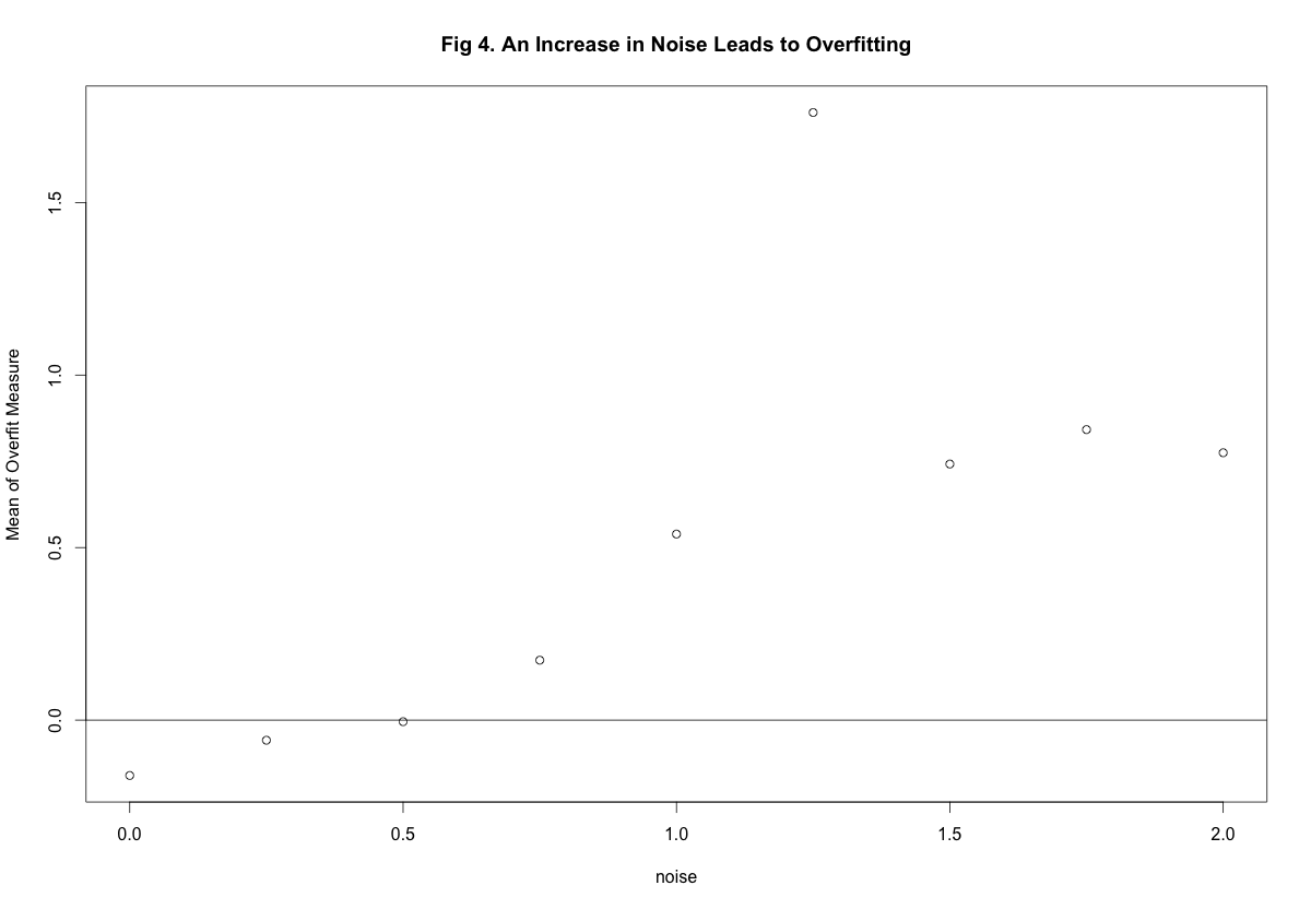
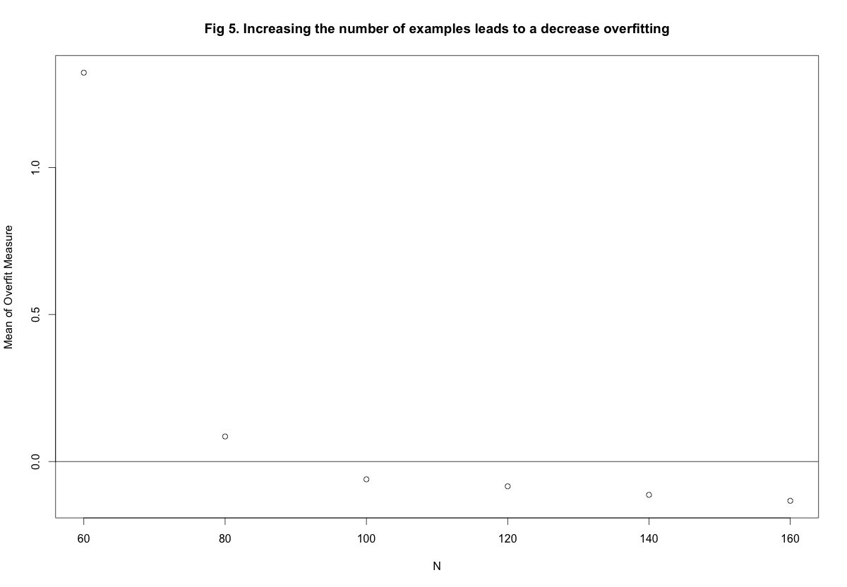
Figure 5 shows the results of varying the number of examples with \(\sigma^2 = 0.5\) and \(Q = 10\). As expected, the more examples we have the more stable the complex \(g_{10}\) model is. In fact if we have more than roughly \(100\) examples, \(g_{10}\) outperforms \(g_2\). Thus an increase number of examples leads to a decrease in the overfit measure.
And lastly we vary degree of \(f\) and fix \(\sigma^2 = .5\) and \(N = 80\). The results can be seen in Figure 6 In this case there is a lot of variability but overall increasing the degree results in a decrease in the overfit measure. However I think this is not so much because of a decrease in variance for \(g_{10}\) as it is a consequence of an increase in bias for \(g_2\).
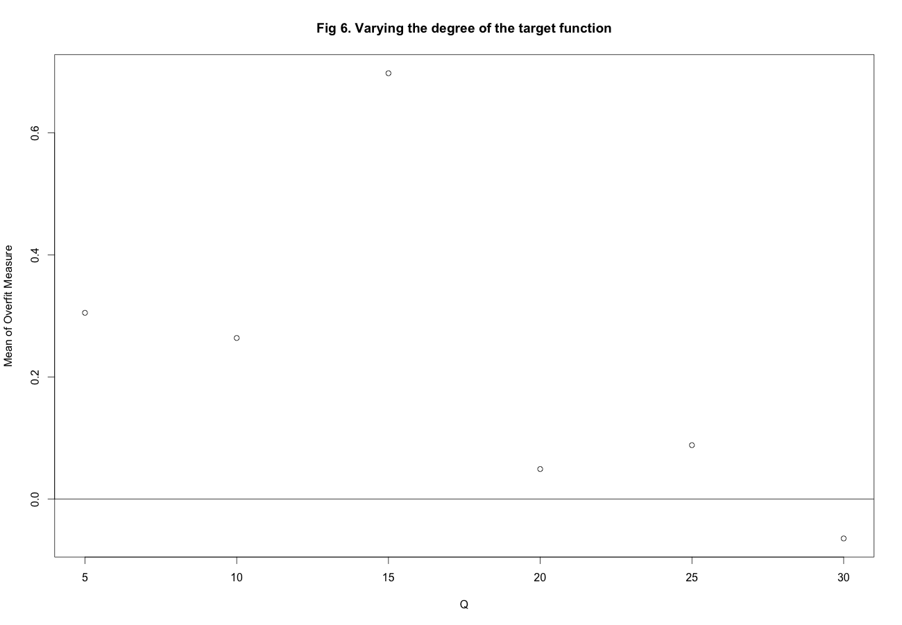
Varying the degree of f for \(N = 80\), \(s^2 = .5\)
Conclusions:
So what can we conclude from our explorations?
-
Generally fitting a second degree polynomial gives a more stable model that is significantly less susceptible to noise than fitting a tenth degree polynomial. The exceptions to this is if you have a lot of training examples and you know the noise is low.
-
An increase in noise leads to an increase in overfitting and higher variance.
-
An increase in the number of training examples leads to a decrease in overfitting. With more examples one should be more confident in using a more flexible and complex model.